2024.06.02 PyTorch Essential Training

1
2
3
4
5
6
7
8
9
Status: Finished
Author: Terezija Semenski
Publishing/Release Date: April 15, 2024
Publisher: Linkedin
Link: https://www.linkedin.com/learning/pytorch-essential-training-deep-learning-23753149/deep-learning-with-pytorch?resume=false&u=3322
Type: Courses
Tags: AI
Start Date: June 1, 2024
End Date: June 2, 2024

Use Google Colab: https://colab.research.google.com/

https://colab.research.google.com/drive/1VHaPSHXGrLlJ5dzC628OVogfY4f8w2mZ

Tensors

Introduction to Tensors

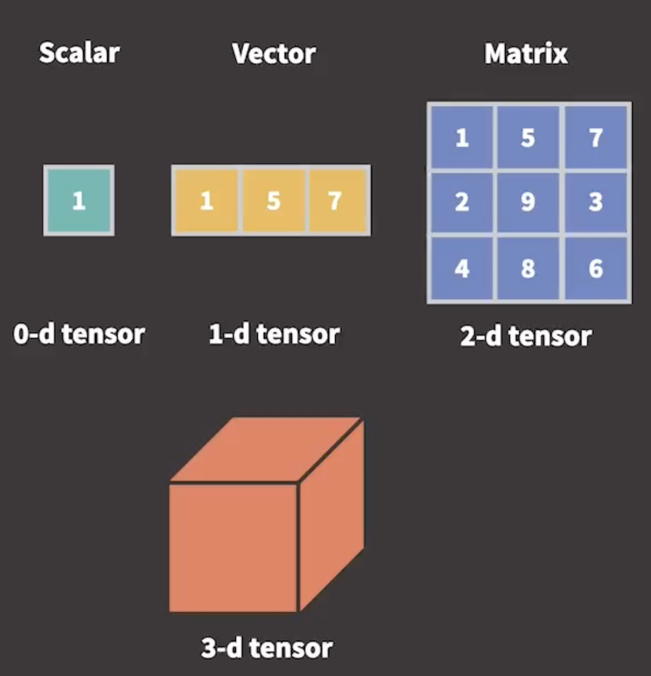
We can think Tensor is generalizations of scalars, vectors, and matrices to any dimension
01

  • Tensor vs ndarray

    Advantages of Tensors

    • Tensor operations are performed significantly faster using GPUs
    • Tensors can be stored and manipulated at scale using distributed processing on multiple CPUs and GPUs and across multiple servers
    • Tensors keep track of the graph of computations that created them

Creating a tensor CPU example

1
2
3
4
5
6
7
8
9
import torch

first_tens = torch.tensor([[12, 10, 11, 9],[13, 15, 14, 16]])
second_tens = torch.tensor([[1, 2, 3, 4], [5, 6, 7, 8]])

add_tens = first_tens + second_tens

print(add_tens)
print(add_tens.size())

output:

1
2
3
tensor([[13, 12, 14, 13],
[18, 21, 21, 24]])
torch.Size([2, 4])
1
2
3
sub_tens = first_tens - second_tens
print(sub_tens)
print(sub_tens.size())

output:

1
2
3
tensor([[11,  8,  8,  5],
[ 8, 9, 7, 8]])
torch.Size([2, 4])

Creating tensors GPU example

1

2

1
2
3
4
5
6
7
8
9
10
11
12
13
14
15
16
import torch

print(torch.__version__)

# output:
# 2.3.0+cu121

if torch.cuda.is_available():
device = "cuda"
else:
device = "cpu"

print(device)

# output:
# cuda
1
2
3
4
5
tens_a = torch.tensor([[10, 11, 12, 13], [14, 15, 16, 17]], device=device)
tens_b = torch.tensor([[18, 19, 20, 21], [22, 23, 24, 25]], device=device)

multi_tens = tens_a * tens_b
print(multi_tens)

output:

The result is also allocated in GPU. The cuda:0 means the first GPU is used. In the case our device contains multiple GPUs, this way, we can controle which GPU is being used.

1
2
tensor([[180, 209, 240, 273],
[308, 345, 384, 425]], device='cuda:0')

Moving Tensor between GPUs and CPUs

  • By default, all the data are in the CPU

  • When training neural network, which is huge, we prefer to use GPU for faster training

  • Transfer the data from the CPU to the GPU

  • After the training, the output tensors are produced in GPU

  • The output data requires preprocessing

  • Some preprocessing libraries don’t support tensors and expect a NumPy array

  • NumPy supports only data in the CPU; we need to move the data from the CPU to the GPU

  • Moving Tensors from CPU to GPU

    1
    2
    3
    4
    5
    6
    7
    8
    # 1st way
    Tensor.cuda()

    # 2nd way
    Tensor.to("cuda")

    # 3rd way
    Tensor.to("cuda:0")
  • Moving Tensors from GPU to CPU

    1
    2
    3
    4
    5
    # 1st case Tensor with required_grad = False
    Tensor.cpu()

    # 2nd case Tensor with required_grad = True
    Tensor.detach().cpu()

Creating Tensors

Different ways to create tensors

http://pytorch.org/docs/stable/torch.html

1
2
3
4
5
6
7
8
9
import torch
import numpy as np

# initialize a tensor from a Python list
tensor_from_list = torch.tensor([1, 2, 3, 4, 5])
# initialize a tensor from a tuple
tensor_from_tuple = torch.tensor((6, 7, 8, 9, 10))
print("Tensor from list:", tensor_from_list)
print("Tensor from tuple:", tensor_from_tuple)
1
2
3
# initialize a tensor from a ndarry
tensor_from_array = torch.tensor(np.array([11, 12, 13, 14, 15]))
print("Tensor from array:", tensor_from_array)
  • Different functions for creating tensors

    torch.empty(), torch.ones(), torch.zeros()

    1
    2
    3
    4
    5
    6
    tensor_emp = torch.empty(3, 4)
    print("tensor_emp :", tensor_emp)
    tensor_zeros = torch.zeros(3, 4)
    print("tensor_zeros :", tensor_zeros)
    tensor_ones = torch.ones(3, 4)
    print("tensor_ones :", tensor_ones)

    torch.rand(), torch.randn(), torch.randint()

    • uniform distribution: 均匀分布
    • normal distribution: 正态分布
    1
    2
    3
    4
    5
    6
    7
    8
    9
    10
    11
    12
    # tensors initialized by size with random values
    # returns a tensor filled with random numbers from a uniform distribution
    tensor_rand_un = torch.rand(4, 5)
    print("tensor_rand_un :", tensor_rand_un)

    # returns a tensor filled with random numbers from a normal distribution
    tensor_rand_norm = torch.randn(4, 5)
    print("tensor_rand_norm :", tensor_rand_norm)

    # returns a tensor filled with random integers generated uniformly (from 5 to 10)
    tensor_rand_int = torch.randint(5, 10, (4, 5))
    print("tensor_rand_int :", tensor_rand_int)

    output:

    1
    2
    3
    4
    5
    6
    7
    8
    9
    10
    11
    12
    tensor_rand_un : tensor([[0.8624, 0.2577, 0.8981, 0.7393, 0.1189],
    [0.1564, 0.9084, 0.1446, 0.2822, 0.2021],
    [0.7456, 0.3061, 0.0126, 0.9152, 0.3011],
    [0.1059, 0.9894, 0.9812, 0.8815, 0.9442]])
    tensor_rand_norm : tensor([[-1.1702, 1.5030, -1.2549, -0.1946, 0.9323],
    [ 0.3549, -0.2362, 0.2905, 0.6290, -0.4099],
    [-1.1625, 1.6882, 0.6824, -0.3181, 0.8423],
    [-0.8305, -0.5503, 0.0125, 1.0829, -0.5804]])
    tensor_rand_int : tensor([[7, 6, 5, 7, 9],
    [7, 8, 9, 7, 6],
    [7, 5, 6, 6, 5],
    [9, 9, 7, 6, 8]])
    1
    2
    3
    # initialize a tensor of ones
    tensor_ones = torch.ones_like(tensor_rand_int)
    print(tensor_ones)

    output

    1
    2
    3
    4
    tensor([[1, 1, 1, 1, 1],
    [1, 1, 1, 1, 1],
    [1, 1, 1, 1, 1],
    [1, 1, 1, 1, 1]])

Tensor attributes

Knowing device location, datatype, dimension, and rank is very important

1
2
3
import torch

first_tensor = torch.tensor([1,2,3,4,5,6])

torch.device indicates the tensor’s device location

1
2
first_tensor.device
# device(type='cpu')

torch.dtype indicates the tensor’s data type

1
2
first_tensor.dtype
# torch.int64

torch.shape shows the tensor’s dimensions

1
2
first_tensor.shape
# torch.Size([6])

torch.ndim identifies the number of a tensor’s dimensions or rank

1
2
first_tensor.ndim
# 1

Tensor data types

Integer data type tensor

1
2
3
4
#@title Integer data type tensor
int_tensor = torch.tensor([1, 2, 3, 4, 5], dtype=torch.int8)
int_tensor.dtype
# torch.int8

Float data type tensor

1
2
3
4
#@title Float data type tensor
float_tensor = torch.tensor([1, 2, 3, 4, 5], dtype=torch.float32)
float_tensor.dtype
# torch.float32

Short data type tensor

1
2
3
4
#@title Short data type tensor
short_tensor = torch.tensor([1, 2, 3, 4, 5], dtype=torch.int16)
short_tensor.dtype
# torch.int16

Casting a tensor to a new data type (1st way)

1
2
3
4
#@title Casting a tensor to a new data type (1st way)
int_tensor = int_tensor.float()
int_tensor.dtype
# torch.float32

Casting a tensor to a new data type (2nd way)

1
2
3
4
#@title Casting a tensor to a new data type (2nd way)
last_tensor = short_tensor.to(dtype=torch.int8)
last_tensor.dtype
# torch.int8

Creating tensors from random samples

1
2
torch.manual_seed(111) # fixed seed
torch.rand(3, 3)

Creating tensors like other tensors

torch.zeros_like(), torch.ones_like(), torch.rand_like()

1
torch.full((4, 5), 5) # a array with all 5

Manipulate Tensors

Tensor operations

Indexing and slicing of tensors is the same way with NumPy

1
2
3
4
5
6
#@title Indexing 1-dim tensor example
one_dim_tensor = torch.tensor([1, 2, 3, 4, 5, 6])
print(one_dim_tensor[2])
print(one_dim_tensor[2].item())
# tensor(3)
# 3
1
2
3
4
#@title Slicing 1-dim tensor example
# [start:end:step]
one_dim_tensor[1:3]
# tensor([2, 3])
1
2
3
4
5
#@title Indexing 2-dim tensor example
two_dim_tensor = torch.tensor([[1, 2, 3, 4, 5, 6], [7, 8, 9, 10, 11, 12],
[13, 14, 15, 16, 17, 18], [19, 20, 21, 22, 23, 24]])
two_dim_tensor[1][3]
# tensor(10)
1
2
3
4
5
#@title Slicing 2-dim tensor example
print("first three elements of the 1st row: ", two_dim_tensor[0, 0:3])
print("first four elements of the 2nd row: ", two_dim_tensor[1, 0:4])
# first three elements of the 1st row: tensor([1, 2, 3])
# first four elements of the 2nd row: tensor([ 7, 8, 9, 10])
1
2
3
#@title Use indexing to extract the data that meets some criteria
two_dim_tensor[two_dim_tensor<11]
# tensor([ 1, 2, 3, 4, 5, 6, 7, 8, 9, 10])
1
2
3
4
5
6
7
8
9
10
11
12
13
#@title Combining tensors 维度增加
torch.stack((two_dim_tensor, two_dim_tensor))

# output
tensor([[[ 1, 2, 3, 4, 5, 6],
[ 7, 8, 9, 10, 11, 12],
[13, 14, 15, 16, 17, 18],
[19, 20, 21, 22, 23, 24]],

[[ 1, 2, 3, 4, 5, 6],
[ 7, 8, 9, 10, 11, 12],
[13, 14, 15, 16, 17, 18],
[19, 20, 21, 22, 23, 24]]])
1
2
3
4
5
6
7
8
9
10
11
12
13
14
15
16
17
18
#@title Concatenation 维度不变,shape增大

tensorA = torch.tensor([[1, 2, 3, 4], [5, 6, 7, 8]])
tensorB = torch.tensor([[9, 10, 11, 12], [13, 14, 15, 16]])

print("Vertically concate tensorA and tensorB: (default: dim=0)")
torch.cat([tensorA, tensorB])

print("Horizontally concate tensorA and tensorB: (default: dim=1)")
torch.cat([tensorA, tensorB], dim=1)

# output
tensor([[ 1, 2, 3, 4],
[ 5, 6, 7, 8],
[ 9, 10, 11, 12],
[13, 14, 15, 16]])
tensor([[ 1, 2, 3, 4, 9, 10, 11, 12],
[ 5, 6, 7, 8, 13, 14, 15, 16]])
1
2
3
4
5
#@title Splitting tensors
first_tensor, second_tensor, third_tensor, fourth_tensor = torch.unbind(two_dim_tensor)
print(first_tensor, second_tensor, third_tensor, fourth_tensor)

# tensor([1, 2, 3, 4, 5, 6]) tensor([ 7, 8, 9, 10, 11, 12]) tensor([13, 14, 15, 16, 17, 18]) tensor([19, 20, 21, 22, 23, 24])
1
2
3
4
5
6
7
8
9
10
#@title Splitting 2-dim tensor
torch.unbind(two_dim_tensor, dim=1)

# output
(tensor([ 1, 7, 13, 19]),
tensor([ 2, 8, 14, 20]),
tensor([ 3, 9, 15, 21]),
tensor([ 4, 10, 16, 22]),
tensor([ 5, 11, 17, 23]),
tensor([ 6, 12, 18, 24]))

Mathematical functions

Built-In Math Functions

  • Pointwise operation

  • Reduction functions

  • Comparison function

  • Linear algebra operation

  • Spectral and other math computations

  • Pointwise operation

    Perform an operation on each point in the tensor individually and return a new tensor

    • Basic math functions: add(), mul(), div(), neg(), and true_divide()
    • Functions for truncation: ceil(), clamp(), floor(), etc.
    • Logical function
    • Trigonometry function (三角函数)
  • Reduction Operations

    Reduce numbers down to a single number or a smaller set of numbers

    • Results in reducing the dimensionality or rank of the tensor
    • Include statistical functions such as mean, median, mode, etc.
  • Comparison Functions

    • Compare all the values within a tensor or compare values of two different tensors
    • Functions to find the minimum or maximum value, sort tensor values, test tensor status or condition, and similar
  • Linear Algebra Functions

    torch.mm(), torch.matmul(), torch.bmm()

    • Enable matrix operations and are essential for deep-learning computations
    • Functions for matrix computations and tensor computations
  • Spectral Operations

    Useful for data transformations or analysis

1
2
3
4
5
6
7
8
9
10
11
#@title Basic math function
a = torch.tensor([10, 2, 8, 6, 4])
b = torch.tensor([1, 2, 4, 3, 1])
print('adding tensors a and b:', a.add(b)) # 等价于 a+b
print('multiplying tensors and b:', a.mul(b)) # a*b
print('dividing tensor and b:', a.div(b)) #a/b

#output
adding tensors a and b: tensor([11, 4, 12, 9, 5])
multiplying tensors and b: tensor([10, 4, 32, 18, 4])
dividing tensor and b: tensor([10., 1., 2., 2., 4.])
1
2
3
4
5
6
7
8
9
10
11
12
13
14
#@title Reduction functions
c = torch.tensor([[20., 14., 11., 8.], [3., 19., 14., 6.]])
print("Mean of the tensor c:", torch.mean(c))
print("Median of the tensor c:", torch.median(c))
print("Model of the tensor c:", torch.mode(c))
print("Standard deviation of the tensor c:", torch.std(c))

# output
Mean of the tensor c: tensor(11.8750)
Median of the tensor c: tensor(11.)
Model of the tensor c: torch.return_types.mode(
values=tensor([8., 3.]),
indices=tensor([3, 0]))
Standard deviation of the tensor c: tensor(6.0341)

Linear algebra operations

http://pytorch.org/docs/stable/linalg.html

PyTorch has a module called torch.linalg that contains a set of built-in algebra functions that are based on BLAS and LAPACK standardized libraries

1
2
3
4
5
6
7
#@title Compute the dot product (scalar) of two 1d dimensions
first_tensor = torch.tensor([1, 2, 3])
second_tensor = torch.tensor([4, 5, 6])

dot_product = torch.matmul(first_tensor, second_tensor)
dot_product
#tensor(32)
1
2
3
4
5
6
7
8
9
10
#@title Compute the matrix-matrix product (2D tensor) of two 2d tensors
first_2d_tensor = torch.tensor([[1, 2, 3], [-1, -2, -3]])
second_2d_tensor = torch.tensor([[-1, -2], [4, 5], [4, 5]])

result_2d_tensor = torch.matmul(first_2d_tensor, second_2d_tensor)
result_2d_tensor

# output
tensor([[ 19, 23],
[-19, -23]])

torch.mm() unlike torch.matmul(), it doesn’t support broadcasting.

1
2
3
4
5
6
7
8
9
10
11
12
13
14
15
#@title Compute the a matrix product of 5 2d tensors 连乘

first_ten = torch.randn(2, 3)
second_ten = torch.randn(3, 4)
third_ten = torch.randn(4, 5)
forth_ten = torch.randn(5, 6)
fifth_ten = torch.randn(6, 7)
torch.linalg.multi_dot((first_ten, second_ten, third_ten, forth_ten, fifth_ten))

# output
tensor([[-5.7800e+00, 1.9394e+01, 2.0585e+00, 6.0236e+01, 3.0810e+01,
-4.3826e+00, 5.4312e+01],
[ 3.9269e+00, -1.3813e-02, -5.8432e-01, 5.1208e+00, 2.3080e+00,
-2.6123e+00, -5.0924e+00]])

1
2
3
4
5
6
7
8
9
10
11
12
13
14
15
16
17
18
19
20
21
22
#@title Computing eigenvalues and eigenvectors 特征值和特征向量

# create a 4x4 square matrix
A = torch.rand(4, 4)

print("Matrix:", A)

eigenvalues, eigenvectors = torch.linalg.eig(A)

print("Eigen Values:", eigenvalues)
print("Eigen Vectors:", eigenvectors)

# output
Matrix: tensor([[8.9473e-02, 1.0631e-01, 2.5981e-01, 5.5447e-01],
[1.9051e-02, 5.7340e-01, 7.4079e-01, 8.2669e-01],
[2.7876e-01, 4.6995e-01, 2.3674e-02, 1.6234e-01],
[2.9856e-04, 5.1959e-01, 7.5827e-01, 3.4576e-01]])
Eigen Values: tensor([ 1.5377+0.0000j, 0.0979+0.0000j, -0.3016+0.2724j, -0.3016-0.2724j])
Eigen Vectors: tensor([[ 0.3142+0.0000j, 0.8435+0.0000j, 0.0867-0.3980j, 0.0867+0.3980j],
[ 0.7153+0.0000j, -0.4333+0.0000j, 0.2588-0.2641j, 0.2588+0.2641j],
[ 0.3363+0.0000j, 0.3132+0.0000j, -0.6401+0.0000j, -0.6401-0.0000j],
[ 0.5258+0.0000j, -0.0509+0.0000j, 0.3846+0.3739j, 0.3846-0.3739j]])

Automatic differentiation (Autograd)

03

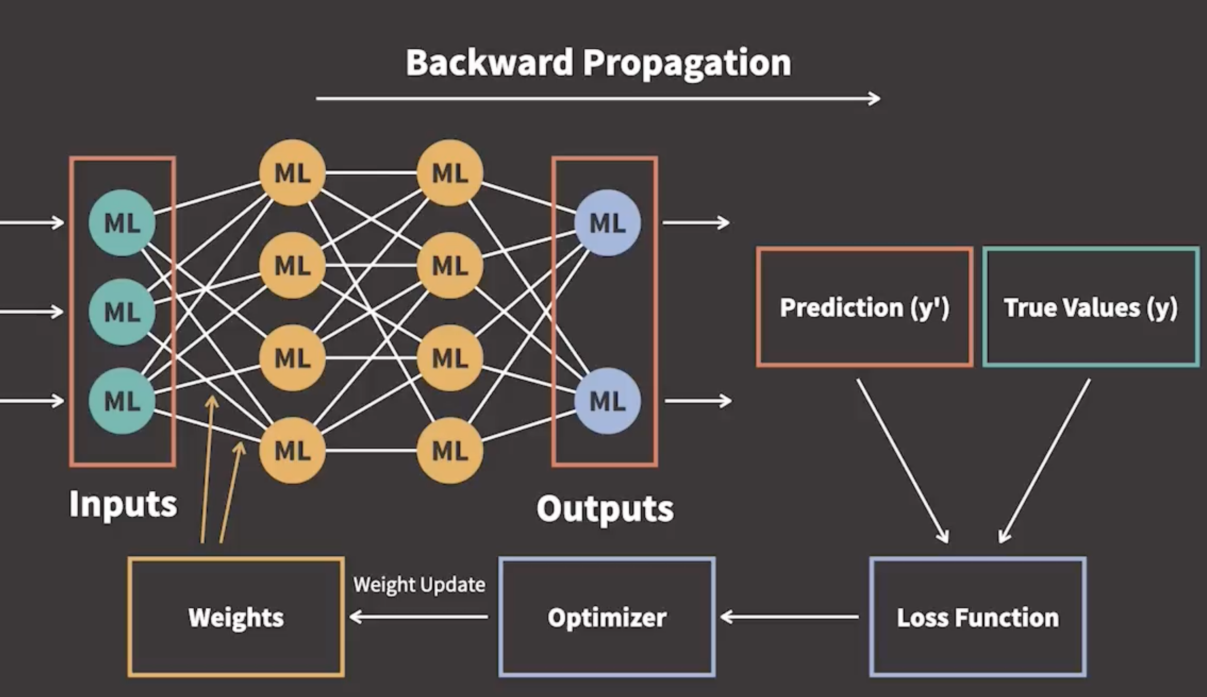
  • After we find the loss function, we calculate the derivative of the loss function in terms of the parameters
  • We iteratively update the weight parameters accordingly so that the loss function returns the smallest possible loss
  • This step is called iterative optimization, as we use an optimizer to perform the update of parameters
  • This process is called gradient-based optimization

Automatic differentiation is a set of techniques that allow us to compute gradients for arbitrary complex loss functions efficiently. (自动求偏导)

Numerical Differentiation

  • Follows the definition of derivative
  • A derivative of y with respect to x defines the rate of change of y with respect to x

$$
\begin{equation} \frac{\partial y}{\partial x} = \frac{f(x+\Delta x)-f(x)}{\Delta x}\end{equation}
$$

Cons of Numerical Differentiation:

  • The computational costs, which increase as we increase the number of parameters in the loss function
  • The truncation errors
  • The round-off errors

Symbolic Differentiation

  • Used in calculus
  • Using a set of rules, meaning a set of formulas that we can apply to the loss function to get the gradients
  • The derivate of a function $f(x) = 3x^2-4x+5$
  • When we apply the symbolic rules, we get $f’(x)=6x-4$

Cons of Symbolic Differentiation:

  • Is limited to the already defined symbolic differentiation rules
  • It can’t be used for differentiating a given computational procedure
  • The computational costs, as it can lead to an explosion of symbolic terms

Automatic Differentiation

refer: computation graph

  • Every complex function can be expressed as a composition of elementary functions
  • For those elementary functions, we could apply symbolic differentiation, which would mean storing and manipulating symbolic forms of derivatives
  • By using automatic differentiation, we don’t have to go through the process of simplifying the expressions
  • Instead, evaluate a given set of values
  • Another benefit of automatic differentiation is that our function can contain if-else statements, for loops, or recursion.
1
2
3
4
#@title Define tensors
x = torch.autograd.Variable(torch.tensor([2.]), requires_grad=True)
y = torch.autograd.Variable(torch.tensor([1.]), requires_grad=True)
z = torch.autograd.Variable(torch.tensor([5.]), requires_grad=True)

Compute gradients

1
2
3
4
5
6
7
8
9
10
11
12
13
14
15
16
17
18
19
#@title Compute gradients
# compute a
a = x - y

# define the function f
f = z * a

# compute gradients
f.backward()

# print the gradient value
print("Gradient value for x:", x.grad)
print("Gradient value for y:", y.grad)
print("Gradient value for z:", z.grad)

# output
Gradient value for x: tensor([5.])
Gradient value for y: tensor([-5.])
Gradient value for z: tensor([1.])

Split tensors to form new tensor

The split function enables you to split tensor given the size of the part

The chunk function enables you to split a tensor into a give number of parts

  • Tensor.chunk(chunks=4, dim=0)
  • Tensor.chunk(chunks=4)
  • Tensor.split([5, 3], dim=0)
  • Tensor.split([4, 6, 6])

Developing a Deep Learning Model

Introduction to the DL training

Data preparation

  • The first step in developing a deep learning model
  • Consists of loading the data, applying transforms, and batching the data using PyTorch’s built-in capabilities
  • Use Python library called Torchvision; it has classes that support computer vision
  • tochvision.datasets module provides several subclasses to load image data from standard datasets such as our CIFAR-10 dataset

Data loading

1
2
3
4
5
6
7
#@title Import libraries and dataset
import torch
from torchvision.datasets import CIFAR10
from keras.datasets import cifar10
from matplotlib import pyplot

train_data = CIFAR10(root="./train/", train=True, download=True)
1
2
3
4
5
6
7
8
9
#@title Load dataset
(trainX, trainy), (testX, testy) = cifar10.load_data()
# summarize loaded dataset
print("Train: X=%s, y=%s" % (trainX.shape, trainy.shape))
print("Test: X=%s, y=%s" % (testX.shape, testy.shape))

#output
Train: X=(50000, 32, 32, 3), y=(50000, 1)
Test: X=(10000, 32, 32, 3), y=(10000, 1)
1
2
3
4
5
6
7
8
9
#@title Display images
# plot first 16 images
for i in range(16):
# define subplot
pyplot.subplot(4, 4, i+1)
# plot raw pixel data
pyplot.imshow(trainX[i])
# show the figure
pyplot.show()
1
2
3
4
5
6
7
#@title Examine the training dataset
print(train_data.data.shape)
print(train_data.class_to_idx)

# output
(50000, 32, 32, 3)
{'airplane': 0, 'automobile': 1, 'bird': 2, 'cat': 3, 'deer': 4, 'dog': 5, 'frog': 6, 'horse': 7, 'ship': 8, 'truck': 9}
1
2
3
4
5
6
7
8
9
10
11
12
13
14
15
16
17
18
19
20
21
22
#@title Check the class labels
for i in range(16):
data, label = train_data[i]
print("Picture: " + str(i+1) + ", photograph: ", train_data.classes[label])

# output
Picture: 1, photograph: frog
Picture: 2, photograph: truck
Picture: 3, photograph: truck
Picture: 4, photograph: deer
Picture: 5, photograph: automobile
Picture: 6, photograph: automobile
Picture: 7, photograph: bird
Picture: 8, photograph: horse
Picture: 9, photograph: ship
Picture: 10, photograph: cat
Picture: 11, photograph: deer
Picture: 12, photograph: horse
Picture: 13, photograph: horse
Picture: 14, photograph: bird
Picture: 15, photograph: truck
Picture: 16, photograph: truck

Data transforms

1
2
3
4
5
6
7
8
9
10
11
12
13
14
15
#@title Import and transform for training data set
from torchvision import transforms
from torchvision.datasets import CIFAR10
train_data_path = "./train/"
train_transforms = transforms.Compose([
transforms.Resize(64),
transforms.ToTensor(),
transforms.Normalize(
mean=(0.4914, 0.4822, 0.4465),
std=(0.2023, 0.1994, 0.2010))])

training_data = CIFAR10(train_data_path,
train=True,
download=True,
transform=train_transforms)
1
2
#@title Training data of first image
print(training_data[0])
1
2
3
4
5
6
7
(tensor([[[-1.2854, -1.3629, -1.5180,  ...,  0.4981,  0.4593,  0.4399],
[-1.4986, -1.5761, -1.7312, ..., 0.3430, 0.3236, 0.3236],
[-1.9057, -1.9832, -2.1383, ..., 0.0522, 0.0522, 0.0716],
...,
[-0.2509, -0.4655, -0.9142, ..., -1.3239, -1.3629, -1.3629],
[-0.0558, -0.1923, -0.4850, ..., -0.8752, -0.9532, -0.9922],
[ 0.0418, -0.0558, -0.2704, ..., -0.6411, -0.7581, -0.8167]]]), 6)
1
2
3
4
5
6
7
8
9
10
11
12
13
14
15
16
#@title Defining transform for testing data set
test_data_path = "./test/"
test_transforms = transforms.Compose([
transforms.ToTensor(),
transforms.Normalize(
mean=(0.4914, 0.4822, 0.4465),
std=(0.2023, 0.1994, 0.2010)
)
])

test_data = CIFAR10(test_data_path,
train=False,
download=True,
transform=test_transforms)

print(test_data)

Data batching

  • A data loader feeds data from the dataset into the neural network
  • At the core of PyTorch data loading utility is the torch.utils.data.DataLoader class
  • It represents a Python iterable over a dataset, with support for:
    • Map-style and iterable-style datasets
    • Customizing data loading order
    • Automatic batching
    • Single and multi-process data loading
  • The neural network trains best with batches of data
  • Instead of using the complete dataset in one training pass, we use mini batches, usually 64 or 128 samples
  • Smaller batches require less memory than the entire dataset, resulting in more efficient and accelerated training
  • DataLoader has, by default, a batch_size of 1
  • batch_size represents a number of images that go through the network before we train and update it
1
2
3
4
5
6
7
8
9
10
11
12
13
14
15
16
17
18
19
20
21
22
23
24
25
26
27
28
29
30
31
32
33
34
35
from torchvision import transforms
from torchvision.datasets import CIFAR10
from torch.utils.data import DataLoader
train_data_path = "./train/"
test_data_path = "./test/"

train_transforms = transforms.Compose([
transforms.Resize(64),
transforms.ToTensor(),
transforms.Normalize(
mean=(0.4914, 0.4822, 0.4465),
std=(0.2023, 0.1994, 0.2010))])

training_data = CIFAR10(train_data_path,
train=True,
download=True,
transform=train_transforms)

test_transforms = transforms.Compose([
transforms.ToTensor(),
transforms.Normalize(
mean=(0.4914, 0.4822, 0.4465),
std=(0.2023, 0.1994, 0.2010)
)
])

test_data = CIFAR10(test_data_path,
train=False,
download=True,
transform=test_transforms)

batch_size = 16
train_data_loader = DataLoader(training_data, batch_size=batch_size, shuffle=True)
test_data_loader = DataLoader(test_data, batch_size=batch_size, shuffle=False)

Model development and training

1
2
3
4
5
6
7
8
9
10
#@title Import libraries and dataset
from torchvision import transforms
from torchvision.datasets import CIFAR10
from torch.utils.data import DataLoader
from torch.utils.data import random_split
from torchvision import models
from torch import optim
import torch.nn as nn
import torch.optim as optim
import torch.nn.functional as F
1
2
3
4
5
6
7
8
9
10
11
12
13
14
15
16
17
18
19
20
#@title Define neural network, init and forward functions
class Net(nn.Module):
def __init__(self):
super(Net, self).__init__()
self.conv1 = nn.Conv2d(3, 6, 5)
self.pool = nn.MaxPool2d(2, 2)
self.conv2 = nn.Conv2d(6, 16, 5)
self.fc1 = nn.Linear(16*5*5, 120)
self.fc2 = nn.Linear(120, 84)
self.fc3 = nn.Linear(84, 10)

def forward(self, x):
x = self.pool(F.relu(self.conv1(x)))
x = self.pool(F.relu(self.conv2(x)))
x = x.view(-1, 16 * 5 * 5)
x = F.relu(self.fc1(x))
x = F.relu(self.fc2(x))
x = self.fc3(x)
return x

1
2
3
4
5
6
#@title Instantiate the Model
net = Net()

# define the loss function and optimizer
criterion = nn.CrossEntropyLoss()
optimizer = optim.SGD(net.parameters(), lr=0.001, momentum=0.9)
1
2
3
4
5
6
7
8
9
10
11
12
13
14
15
#@title Load and transform the data
transform = transforms.Compose([
transforms.ToTensor(),
transforms.Normalize((0.5, 0.5, 0.5), (0.5, 0.5, 0.5))])

traindata = CIFAR10(root="./data", train=True, download=True, transform=transform)

train_set, val_set = random_split(train_data, [40000, 10000])

trainloader = torch.utils.data.DataLoader(train_set, batch_size=4, shuffle=True, num_workers=2)

valloader = torch.utils.data.DataLoader(val_set, batch_size=4, shuffle=True)

testset = CIFAR10(root="./data", train=False, download=True, transform=transform)
testloader = torch.utils.data.DataLoader(testset, batch_size=4, shuffle=False, num_workers=2)
1
2
3
4
5
6
7
8
9
10
11
12
13
14
15
16
17
18
19
20
21
22
23
#@title Train the network
for epoch in range(10): # loop over the dataset multiple times
running_loss = 0.0
for i, data in enumerate(trainloader, 0):
# get the inputs; data is a tuple of [inputs, labels]
inputs, labels = data

# zero the parameter gradients
optimizer.zero_grad()

# forward + backward + optimize
outputs = net(inputs)
loss = criterion(outputs, labels)
loss.backward()
optimizer.step()

# print statistics
running_loss += loss.item()
if i % 2000 == 1999: #print every 2000 mini-batches
print(f'[{epoch+1}, {i + 1: 5d}] loss: {running_loss / 2000: .3f}')
running_loss = 0.0

print('Finish Training')

With validation

1
2
3
4
5
6
7
8
9
10
11
12
13
14
15
16
17
18
19
20
21
22
23
24
25
26
27
28
29
30
31
32
33
34
35
36
37
38
39
#@title Train the network
for epoch in range(10): # loop over the dataset multiple times
net.train() # Set the model to training mode
running_loss = 0.0
for i, data in enumerate(trainloader, 0):
# get the inputs; data is a tuple of [inputs, labels]
inputs, labels = data

# zero the parameter gradients
optimizer.zero_grad()

# forward + backward + optimize
outputs = net(inputs)
loss = criterion(outputs, labels)
loss.backward()
optimizer.step()

# print statistics
running_loss += loss.item()
# if i % 2000 == 1999: #print every 2000 mini-batches
#print(f'[{epoch+1}, {i + 1: 5d}] loss: {running_loss / 2000: .3f}')
#running_loss = 0.0

net.eval() # Set the model evaluation mode for validation
validation_loss = 0.0
correct = 0
total = 0
with torch.no_grad():
for data in valloader:
images, labels = data
outputs = net(images)
loss = criterion(outputs, labels)
validation_loss += loss.item()
_, predicted = torch.max(outputs.data, 1)
total += labels.size(0)
correct += (predicted == labels).sum().item()
print(f'{epoch+1}, Training loss: {running_loss / len(trainloader): .3f}, Validation Loss: {validation_loss / len(valloader)}, Validation Accuracy: {100*correct / total}%')

print('Finish Training')